
last edited on 2020-10-11
Introduction
What's
PyBLD?
PyBLD
Version 3
History
Version
License
Commands
and Functions
Installation
System
Requirements
Install PyBLD
Usage
Tutorial
How
do you implement your C code on PyBLD?
Image manipulation
Note
for person who is already familiar with BLD
ChangeLog
Acknowledgments
Reference
PyBLD is developed to analyze scientific data, especially for analyzing time-cource data and multidimensional data. PyBLD is running on Python, interpreter-type language. Origin of PyBLD is BLD developed by Dr. Richard E Carson [1]. PyBLD is my work to dedicate to Dr. Richard E Carson. PyBLD is still beta stage and you might feel PyBLD is not fully functioned. This is not a sake of BLD but the insufficiency of PyBLD is my responsibility. Please send me any comments, which make PyBLD grow.
Python is now moving toward version 3 and PyBLD must evolve for Python3. There are several differences between Python2 and Python3, and PyBLD version 3 is just started, and there may be several incompatibility issues. So please let me know if you find any problems and bugs.
When I was
working at NIH in USA from 1997 to 1999, Dr Richard E Carson was my
supervisor. I learned many things from him and BLD is one thing I
cannot forget. Before I started using BLD, I used to program
everything in C. Although BLD is slower than C, BLD is very
convenient n many cases because of interpreter language (people who
knows Matlab or IDL understand the benefit of the interpreter
language).
After I came back to Japan, I missed BLD very much,
however it was not easy to build BLD environment in Japan. BLD was
developed on VMS OS, and I don't have any VMS computer. So Python.
Soon after starting to learn Python, I realized how powerful python
is, i.e. interpreter, objected-oriented, easy to learn, easy to read
programs etc, and I finally decided to develop BLD environment on
Python.
Current version of PyBLD is 3.3. This version is for Python3. If you prefer to use Python2, let me know, the PyBLD version 2 is still active and I can offer the source codes.
PyBLD is
free software; you can redistribute it and/or modify it under the
terms of the GNU General Public License as published by the Free
Software Foundation; either version 2, or (at your option) any later
version.
PyBLD is distributed in the hope that it will be
useful, but WITHOUT ANY WARRANTY; without even the implied warranty
of MERCHANT ABILITY or FITNESS FOR A PARTICULAR PURPOSE. See
the GNU General Public License for more details.
Here some of commands and functions which PyBLD has
input - read data from text file
output - write data to text file
mullin - linear regression of one dependent variable against any number of independent variables
polfit - polynomial fit
fit - non-linear least squared fitting to user-defined function
save - save variables
recall - recall variables
interpolate - interpolate data
integrate - integrate data
conv_exp - convolution with exponential curve
plot - plot data
gaus - Gaussian filter
spline - Spline fit
Please see pybld and bldanaimg helps generated by pydoc.
Computer running Unix OS (Linux, Solaris have been confirmed to run PyBLD. Probably another Unix machine should be fine with minor modification) or Window OS or MacOS-X.
Python (3.4 or greater) - interpreter type script language. Core of PyBLD
NumPy (1.0 or greater) - N-dimensional Array manipulations. Matrix calculation and several useful mathematical definitions
SWIG (1.1p5) - optional. wrapper generator from raw C code to Python script language. If you want to install own module by C, or C++ you might want to have SWIG.
Matplotlib – Since PyBLD version 3.0, matplotlib is default plotting library
grace (5.1.0 or greater) - excellent plotting program which is callable from PYBLD on Linux
gpetview- if you want to display image through PyBLD. This is for you.
setuptools - From version 2.5, I use setuptools instead of distutil. You must install setuptools by pip, easy_install, or most Linux distribution offers package for setuptools
After
installing the above software,
1. Download PyBLD source from
here.
2. Extract sources by tar
xvzf PyBLD-3.3.tar.gz
3. Change source directory as cd
PyBLD-3.3
4.
If you want to develop your own module using SWIG, Type configure
and make
5. Type 'python3 setup.py install'
6(optional). If you
like to use gen_pybld_pass.py, type autoconf and configure
7.
copy bin/pybld and bin/gen_pybld_pass.py into directory where you can
put your executable file (i.e. /usr/local/bin)
8. Edit
.pybld_start (if there is no .pybld_start, please copy pybld_start.py
in the source directory to your HOME directory) in your HOME
directory if you wish. For example, if you like to use grace rather
than matplotlib, give one line as bld.gp_cmd = 'matplotlib' in
.pybld_start.
If you are MS-Windows and Mac user, please install through anaconda3
Conda command is as follows; conda install -c whiroshi pybld
Or you can install PyBLD by pip.
PyBLD uses many functions from Python and Numerical Python(NumPy). So you must learn how to use Python and NumPy before using PyBLD. See the homepages of Python and Numerical Python. You will find several documents including manual and tutorial of Python and NumPy. You can find details of functions in PyBLD in pybld and bldanaimg pydoc files. Please take a look at some examples in 'test' directory of PyBLD source.
(This tutorial is originally from BLD manual)
Example
1
The following example takes a file that has a list of plasma
counts, decay corrects these counts and plots a plasma curve. We have
a data file called xyzzy.dat that looks like
this:
#sample
time raw cpm mid-point count volume(cc) bkg cpm
0 0
115.0
103.78
.3
106.0
0 14 107.5
106.10 .3
106.0
0 29 3469.0
108.40 .3
106.0
0 44 89582.2
109.91 .3
106.0
0 59 230738.8
110.53 .3
106.0
1 15 243964.7
110.98 .3
106.0
1 31 167908.3
111.48 .3
106.0
1 45 132612.9
112.04 .3
106.0
2 00 97756.1
112.70 .3
106.0
2 30 80544.0
113.43 .3
106.0
3 00 76322.6
114.25 .3
106.0
3 30 72798.9
115.09 .3
106.0
4 00 67443.3
116.07 .3
106.0
5 01 60659.1
116.99 .3
106.0
6 04 56647.9
117.96 .3
106.0
8 00 49656.8
119.01 .3
106.0
10 00
44196.7 120.18
.3 106.0
12
00
39301.0 121.44
.3 106.0
15
00
34139.0 122.84
.3 106.0
20
00
31244.2 124.37
.3 106.0
30
00
25280.5 126.12
.3 106.0
57
51
16624.5 128.22
.3 106.0
68
20
14839.0 130.53
.3 106.0
(Note: a line which begins with # is considered a comment line)
We want to
use BLD to take these raw counts and decay correct them back to
injection time. How do we do this?
The first
thing to notice about this data file is that it contains six columns
of data; time in minutes, time is seconds, raw cpm, the mid-point
counting time (the time in minutes between counting time and
injection time), the volume of plasma counted and the
background average for the day.
Type 'pybld' to start PyBLD.
1. to read 'xyzzy.dat', use 'input' command;
timmin,timsec,raw,counttim,vol,bkg = bld.input('xyzzy.dat')
2. to see current variables, use 'var' command
bld.var()
3. we set halflife of F-18 and get decay
corrected counts as follows;
halflife = 109.8
cor1 = (raw - bkg)/vol
newcounts = cor1*(power(2.0,(counttim/halflife)))
newtime=timmin+(timsec/60.0)
4. Finally plot newtime vs
newcounts using 'plot' command
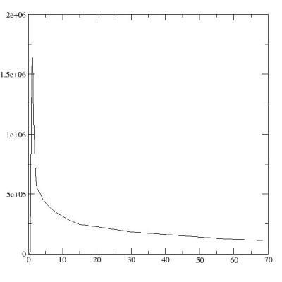
bld.plot(newtime,newcounts)
which shows a graphic window
of grace and you can configure the graph and send to a printer if you
like.
5. Save
newtime and newcounts by 'output' command
bld.output('newcnt.dat',newtime,newcounts)
6. In order
to exit PyBLD, just type control+D
Example
2
This example shows how to fit data (two exponentials) and plot
out the results.
First, create file 'fff.met'
which looks like the following;
#SAMPLE PLASMA EA AQ _% SD FRACTION SD
#TIMES RECOVERED OF EA
0 3.27E6 737880.3 65276.9 98.2 .42 .92 5.8E-4
0.98 161489.6 34267.5 6614.6 101.3 .81 .84 .003
2.98 173878.9 36853.9 7248.1 101.4 .84 .84 .003
5.1 79686.2 14543.9 4773.0 97.0 1.22 .75 .006
7 55556.0 8813.3 4805.0 98.0 1.55 .65 .008
10.25 44051.8 5547.6 5452.0 99.9 1.84 .50 .009
20.5 40964.0 2603.6 7216.8 95.9 1.79 .26 .008
29.95 37302.2 2218.4 4772.8 75.0 1.76 .32 .011
40 33748.0 1510.3 6602.2 96.2 2.15 .19 .010
60.08 31063.6 1117.9 5581.6 86.3 2.27 .17 .012
80.03 27702.3 1125.6 5407.7 94.3 2.54 .17 .012
120 23405.5 780.0 4472.1 89.7 3.06 .15 .016
1. Start
PyBLD by typing 'pybld'
2. Read 'fft.met' as follows;
time,pl,ea,aq,erc,sd_1,fraction,sd_2=bld.input('fff.met')
Selecting eight variables appropriately named, to hold the
columns of data to be read in from the file.
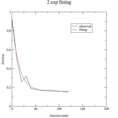
3. We want to fit
time vs fraction as two exponential functions (4 parameters to be
estimated). We create an array which contains initial guess of the
fitting
p = array([0.6,-0.1,0.3,0.0])
We
want to use two exponentials, therefore four parameters are
necessary.
The equation to be used is:
a*exp(b *time) +
c*exp(d*time). We must supply initial guesses for the
parameters a,b,c, and d to start the iterations.
4. Start
fitting using pybld function 'expfit'
res,se=bld.expfit(time,fraction,p)
PyBLD provides
details of each iteration until convergence is reached as follows;
number of parameters = 4
Initial parameter estimates :
Parameter 1 = 0.6
Parameter 2 = -0.1
Parameter 3 = 0.3
Parameter 4 = 0
Initial sum of squares = 0.105581
Iteration 1
Sub-iteration : 0 Sum of squares = 0.0402058
End of sub-iterations
Para 1 = 0.756061 Change = 0.156061 % Chg = 20.6414
Para 2 = -0.0564885 Change = 0.0435115 % Chg = -77.0271
Para 3 = 0.173263 Change = -0.126737 % Chg = -73.1472
Para 4 = -0.000470269 Change = -0.000470269 % Chg = 100
Iteration 1 Sum of squares= 0.0402058
Iteration 2
Sub-iteration : 0 Sum of squares = 0.021275
End of sub-iterations
Para 1 = 0.740184 Change = -0.0158779 % Chg = -2.14512
Para 2 = -0.0740027 Change = -0.0175142 % Chg = 23.6669
Para 3 = 0.198041 Change = 0.0247782 % Chg = 12.5116
Para 4 = -0.00217595 Change = -0.00170568 % Chg = 78.3879
Iteration 2 Sum of squares= 0.021275
.
.
.
Iteration 9
Sub-iteration : 0 Sum of squares = 0.0203654
End of sub-iterations
Para 1 = 0.775023 Change = 8.85232e-07 % Chg = 0.00011422
Para 2 = -0.0716088 Change = 2.05486e-07 % Chg = -0.000286956
Para 3 = 0.16261 Change = -1.10697e-06 % Chg = -0.00068075
Para 4 = -0.000346839 Change = 7.31321e-08 % Chg = -0.0210853
Iteration 9 Sum of squares= 0.0203654
** Convergence has occurred **
Parameter Estimate Standard
Error
1 0.775023 0.0905811
2 -0.0716088 0.0167422
3 0.16261 0.0951439
4 -0.000346839 0.00665002
Std error of the estimate : 0.0504547
Sum of squares : 0.0203654
F value (4,7) : 85.4003
R square : 0.97992
Correlation coefficient : 0.989909
If you don't want to see detail of fitting, you can set variable PYBLD.show = 0.
5. In the
variable 'res', you will see the estimated parameters of the fitting
result. se contains the standard errors of the estimated parameters
from the fit. A matrix is produced from the fit called
PYBLD.corrmat. This is the correlation matrix of the estimated
parameters.
When the fit is completed a new variable
PYBLD.fit_z is created. This contains the fitted curve. You can check
how this fitting works by plotting data with fitted result as
follows;
bld.plot(time,fraction,bld.fit_z)
You can put title and labels of axis and legends on the graph
as follows;
bld.title = '2 exp fitting'
bld.legend='observed','fitting'
bld.xlabel
= 'time(seconds)'
bld.ylabel = 'fraction'
bld.plot(time,fraction,bld.fit_z)
You can
make your own C program which can be called from PyBLD session.
You
must create your C program as follows;
float
*your_function(int *ndim, float *var1, float *var2, .....,int
*num_row, int *num_col) /* you put your variables between 'ndim'
and'num_row' */
{
float *res;
int
npts,i;
npts
= ndim[0]; /* number of element in first variable. second ndim[2],
third ndim[4]....*/
printf("npts
= %d\n",npts);
res
= (float *)malloc(sizeof(float)*npts);
for(i=0;i<npts;i++){
res[i]
= p[0]*x[i] + p[1];
}
*num_row
= npts;
*num_col
= 1;
return
res;
}
gen_pybld_pass.py
generates interface file for Swig and wrapper program between your
program and PyBLD as well as template of makefile for your program.
Original
BLD can handle MIRAGE format images. PyBLD can handle Analyze format
images instead of MIRAGE.
In order to manipulate image in
PyBLD, at first you must make instance of image class as follows;
img
= bld.img()
After that, the instance img can read and write and manipulate
images. For example
img.read('analyze.file')
- read image
img.write('analyze.file')
- write image
img.img
= img.img*2 -
multiple 2
img.view()
-
going to display image by gpetview
Although
PyBLD is tried to be a clone of BLD, there are several differences
between PyBLD and BLD. These differences mainly come from Python
language. Python is written by C language, on the other hand,
original BLD is written by Fortran.
For example,
Array
- the expression of arrays in PyBLD is a[0],a[1],.. and the
corresponding expression in BLD is a(1),a(2),..
Case
sensitive - variables in PyBLD are case sensitive, i.e. A and a
are different.
In addition, you can use several functions and flow controls supported by Python and NumPy which original BLD does not have.
2020-10-11
Version 3.3 some minor bug fix related to interpolate and image
output
2020-01-13 Version 3.2 some minor bug fix related to
saving image, recall
2019-02-11 Version 3.1 some minor bug
fix
2016-09-11 Version 3.0 PyBLD for
Python3
2012-08-13 Version 2.6 some
improvements for bldanaimg
2011-02-08 Version
2.5 bug fix for image header structure. Now img can be saved and
recalled correctly.
2010-07-02 Version 2.4.
img_transform for 4D data
2008-06-27 Version 2.3. zeros function
to prepare new image. output multiarray.
2007-08-14 Version
2.2beta. bug fix in mullin and polfit, get rid of piecies from
Numeric, xmgrace without safemode for saving grace
file
2007-03-20 Version 2.1beta. bug fix for bldanaimg for
swapped image.
2007-01-04 Version 2.0beta. PyBLD for
NumPy
2005-10-21 Version 1.10beta. possible to plot
multi-columns data, error bar. rotate image along x-axis and y-axis.
Byte image transformation.
2004-03-05 Version 1.9beta. Bug fix
for fitting. Clean up several codes. Zooming image. view(number) for
numbering
2004-02-17 Version 1.8beta. Add Affine transformation,
rotate_z for manuplating image. Bug fix for romdom number
generator
2003-07-25 Version 1.7beta. add spline fitting. bug
fix for random. Update web page.
2003-06-28 Version 1.6beta.
bug fix for 2D filter. Graph title and xylabel and legends. several
bug fixes
2003-05-27 Version 1.5beta. add pconv_exp. clean up
polfit,mullin and fit functions
2003-02-27 Version 1.4beta.
patch by Peter McCluskey
2003-01-07 Version 1.3beta. show_flag
for determining detail printing or not. possible to maniplate 4
dimensional image
2002-11-26 Version 1.2beta. Bug fix in
histogram
2002-10-24 Version 1.1beta. rearrange documents.
minor bug fix
2002-08-29 Version 1.0beta. Use distutils
2002-01-28 plot data with different length. give image max and
min by img.max() and img.min(), consider offset of image in
bldimg.py. Check type of int and short in bldutil.py. proper
installation directory. Add example of script interpolation
(interp.py) (version 0.94b)
2001-11-15 Brush-up import_array,
filtering routines, add example17. bldanaimg togpetview() and initial
parameters. (version 0.93b)
2001-07-08 Bug fix in random
routine and fitting routine. add histogram (version 0.92b)
2001-05-15 Lots of modifications for example no fortran
routine, image routine (version 0.91b)
2000-10-30 First public
release (version 0.9a)
I would
like to express my great gratitude to Dr. Richard E. Carson who
originally developed BLD and permits me to re-distribute BLD as
PyBLD.
I would like to appreciate the developers of Python,
NumPy, SWIG.
PyBLD uses datafile.py and grace_np.py
written by Michael Haggerty.
[1] R.E. Carson, S.C. Huang and M.E. Phelps "BLD - a software system for physiological data handling and model analysis", Proceedings of the Fifth Annual Symposium on Computer Applications in Medical Care" pp562-565(1981)
Mail
comments and bug reports to watabe at cyric.tohoku.ac.jp
Hiroshi Watabe
Division
of Radiation Protection & Safety Control,
Cyclotron and
Radioisotope Center,
Tohoku University
6-3 Aoba, Aramaki,
Aoba, Sendai 980-8578 Japan